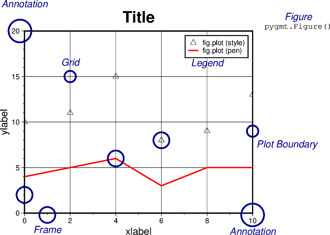
3. Figure elements

The figure below shows the naming of figure elements in PyGMT.

import pygmt
from pygmt.params import Axis, Box, Frame, Position

fig = pygmt.Figure()

x = range(0, 11, 2)
y_1 = [10, 11, 15, 8, 9, 13]
y_2 = [4, 5, 6, 3, 5, 5]

fig.basemap(
    region=[0, 10, 0, 20],
    projection="X10c/8c",
    frame=Frame(
        axes="WSrt",
        title="Title",
        xaxis=Axis(annot=2, tick=1, grid=2, label="xlabel"),
        yaxis=Axis(annot=5, tick=1, grid=5, label="ylabel"),
    ),
)
fig.plot(x=x, y=y_1, style="t0.3c", label="fig.plot (style)")
fig.plot(x=x, y=y_2, pen="1.5p,red", label="fig.plot (pen)")

mainexplain = {"font": "12p,2,darkblue", "justify": "TC", "no_clip": True}
minorexplain = {"font": "10p,8", "justify": "TC", "no_clip": True}
# ============ Figure
fig.text(x=12, y=22, text="Figure", **mainexplain)
fig.text(x=12, y=20.8, text="pygmt.Figure()", **minorexplain)
# ============ x-majorticks
fig.plot(x=10, y=-0.2, style="c1c", pen="2p,darkblue", no_clip=True)
fig.text(x=10, y=-1.6, text="Annotation", **mainexplain)
# ============ y-majorticks
fig.plot(x=-0.2, y=20, style="c1c", pen="2p,darkblue", no_clip=True)
fig.text(x=0, y=23.4, text="Annotation", **mainexplain)
# ============ x-minorticks
fig.plot(x=1, y=-0.2, style="c0.7c", pen="2p,darkblue", no_clip=True)
fig.text(x=1, y=-1.4, text="Frame", **mainexplain)
# ============ y-minorticks
fig.plot(x=0, y=2, style="c0.7c", pen="2p,darkblue", no_clip=True)
# ============ Grid
fig.plot(x=2, y=15, style="c0.5c", pen="2p,darkblue")
fig.text(x=2, y=17, text="Grid", **mainexplain)
# ============ Plot Boundaries
fig.plot(x=10, y=9, style="c0.5c", pen="2p,darkblue", no_clip=True)
fig.text(x=11.5, y=8, text="Plot Boundary", **mainexplain)
# ============ fig.plot (style)
fig.plot(x=6, y=8, style="c0.7c", pen="2p,darkblue")
# ============ fig.plot (pen)
fig.plot(x=4, y=6, style="c0.7c", pen="2p,darkblue")
# ============ Legend
fig.legend()
fig.text(x=8, y=16.9, text="Legend", **mainexplain)

fig.show()

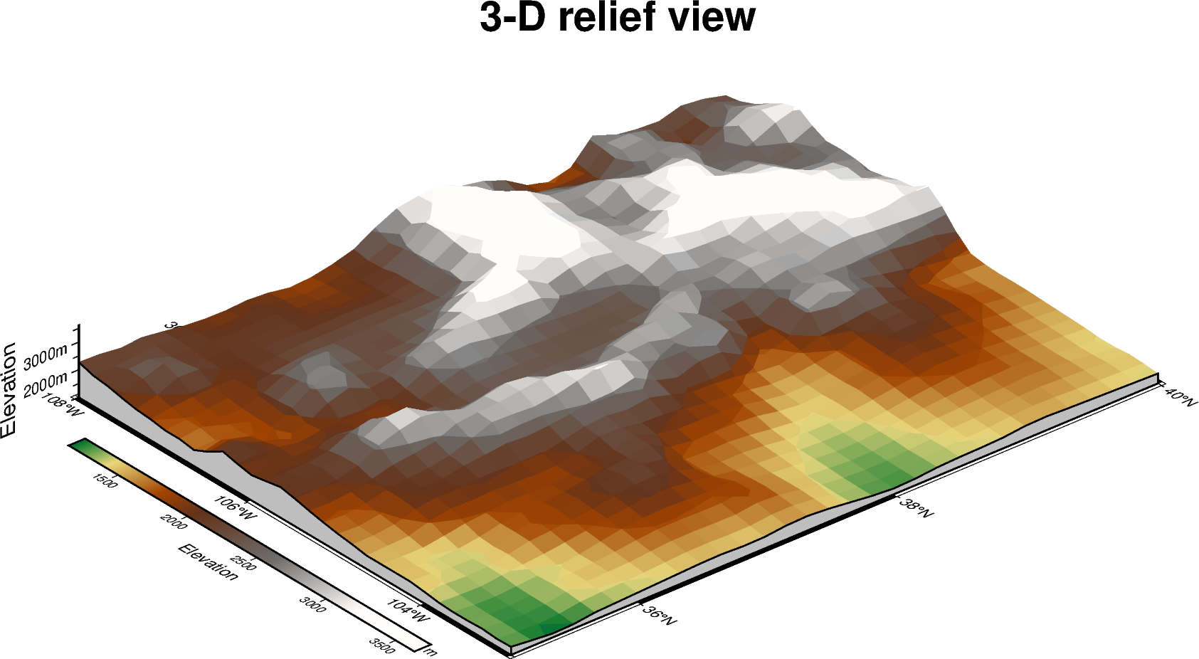
3-D plot example

Figure elements are also important in 3-D views. Here we use a perspective plot of Earth relief and add a title, axis annotations, and a colorbar aligned with the 3-D view.

grid = pygmt.datasets.load_earth_relief(
    resolution="10m", region=[-108, -103, 35, 40]
)

fig = pygmt.Figure()
fig.grdview(
    grid=grid,
    projection="M12c",
    perspective=[130, 30],
    zsize="1.5c",
    surftype="surface",
    cmap="gmt/geo",
    frame=Frame(
        axes="WSnEZ",
        title="3-D relief view",
        xaxis=Axis(annot=True, label="Longitude"),
        yaxis=Axis(annot=True, label="Latitude"),
        zaxis=Axis(annot=1000, tick=500, label="Elevation", unit="m"),
    ),
    plane=1000,
    facade_fill="gray",
)
fig.colorbar(perspective=True, annot=500, label="Elevation", unit="m")
fig.show()

gmtread [NOTICE]: Remote data courtesy of GMT data server oceania [http://oceania.generic-mapping-tools.org]
gmtread [NOTICE]: SRTM15 Earth Relief v2.7 at 10x10 arc minutes reduced by Gaussian Cartesian filtering (52.4 km fullwidth) [Tozer et al., 2019].
gmtread [NOTICE]:   -> Download grid file [3.0M]: earth_relief_10m_g.grd

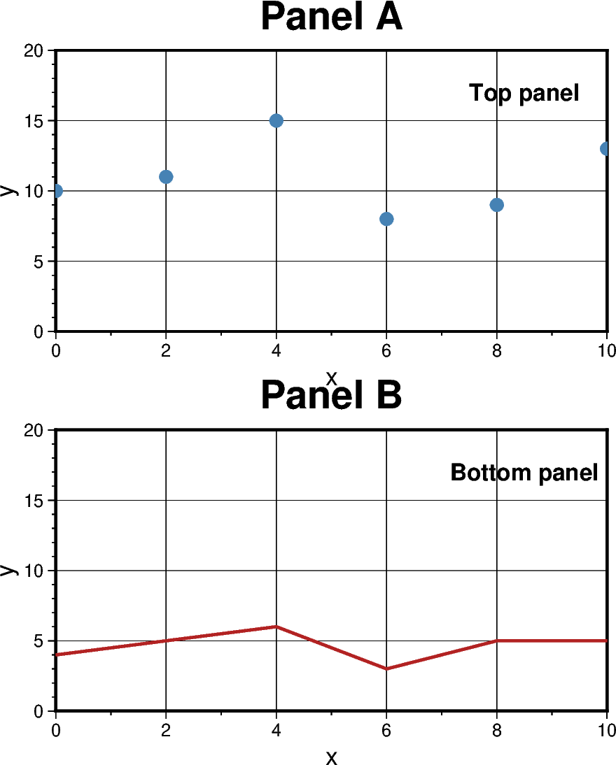
Subplot example

Figure elements can also be organized across multiple panels. The example below uses a 2x1 subplot layout, where each panel has its own title and frame annotations.

fig = pygmt.Figure()
with fig.subplot(
    nrows=2,
    ncols=1,
    figsize=("10c", "12c"),
    frame=Frame(
        axes="WSrt",
        xaxis=Axis(annot=2, tick=1, grid=2, label="x"),
        yaxis=Axis(annot=5, tick=1, grid=5, label="y"),
    ),
    margins="0.4c",
):
    fig.basemap(region=[0, 10, 0, 20], projection="X?", panel=[0, 0], frame="+tPanel A")
    fig.plot(x=x, y=y_1, style="c0.25c", fill="steelblue", panel=[0, 0])
    fig.text(x=8.5, y=17, text="Top panel", font="12p,Helvetica-Bold", panel=[0, 0])

    fig.basemap(region=[0, 10, 0, 20], projection="X?", panel=[1, 0], frame="+tPanel B")
    fig.plot(x=x, y=y_2, pen="1.5p,firebrick", panel=[1, 0])
    fig.text(
        x=8.5,
        y=17,
        text="Bottom panel",
        font="12p,Helvetica-Bold",
        panel=[1, 0],
    )

fig.show()

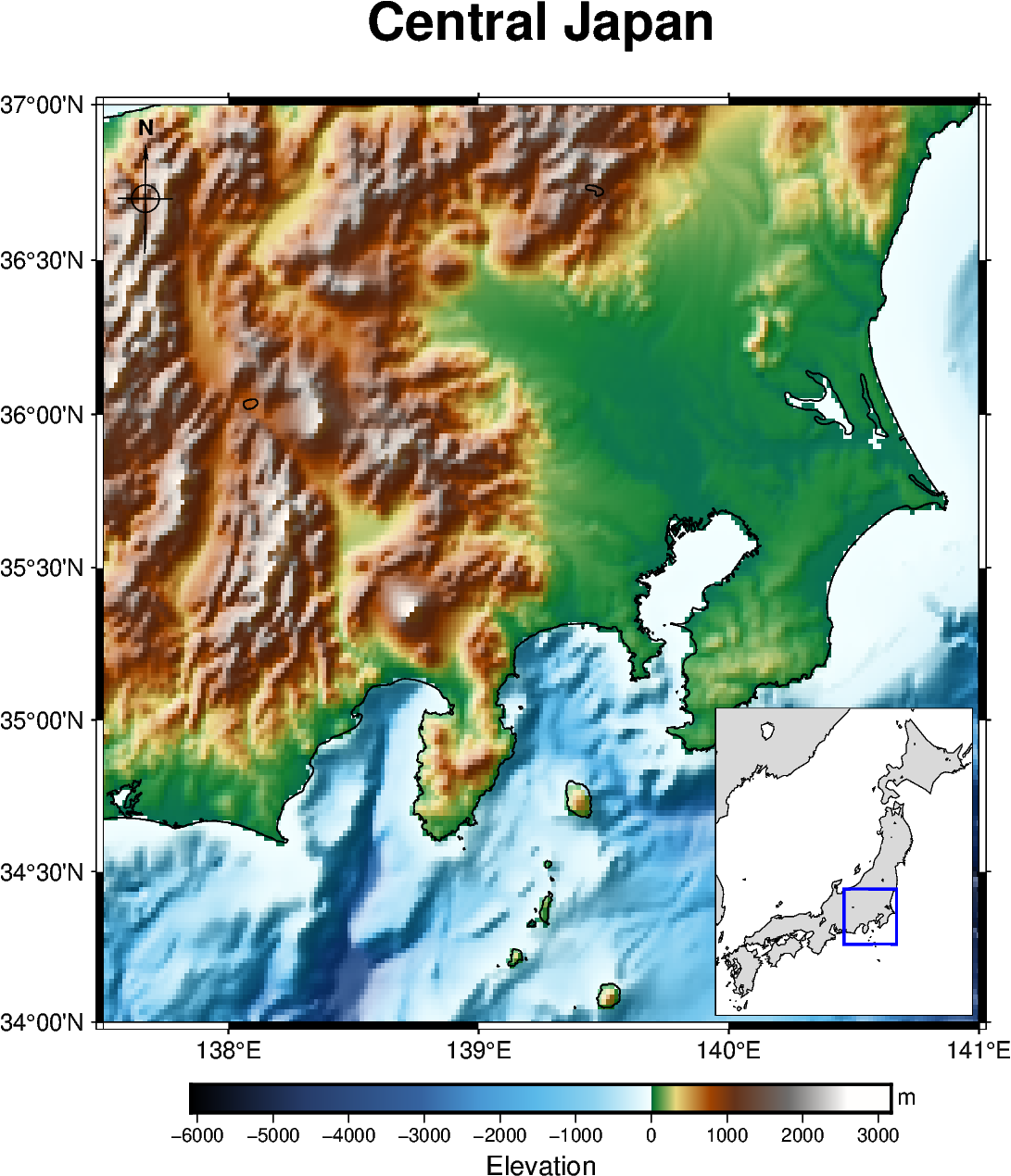
Geographic map example

Figure elements are also commonly used on geographic maps. The example below uses Earth relief as the main map, then adds a colorbar, a directional rose, and an inset map to show where the study area is located in a broader regional context.

region = [137.5, 141, 34, 37]
grid = pygmt.datasets.load_earth_relief(resolution="01m", region=region)

fig = pygmt.Figure()
fig.grdimage(
    grid=grid,
    projection="M12c",
    cmap="gmt/geo",
    shading=True,
    frame=Frame(
        axes="WSne",
        title="Central Japan",
        xaxis=Axis(annot=True, label="Longitude"),
        yaxis=Axis(annot=True, label="Latitude"),
    ),
)
fig.coast(shorelines="0.5p,black")
fig.colorbar(annot=1000, label="Elevation", unit="m")
fig.directional_rose(
    position=Position("TL", offset=0.2),
    width="1.5c",
    labels=True,
)

with fig.inset(
    position=Position("BR", offset=0.1),
    box=Box(fill="white", pen="0.8p"),
    region=[129, 146, 30, 46],
    projection="M3.5c",
):
    fig.coast(land="gray85", water="white", shorelines="0.25p")
    fig.plot(
        data=[[region[0], region[2], region[1], region[3]]],
        style="r+s",
        pen="1p,blue",
    )

fig.show()

grdblend [NOTICE]: Remote data courtesy of GMT data server oceania [http://oceania.generic-mapping-tools.org]
grdblend [NOTICE]: SRTM15 Earth Relief v2.7 at 01x01 arc minutes reduced by Gaussian Cartesian filtering (5.2 km fullwidth) [Tozer et al., 2019].
grdblend [NOTICE]:   -> Download 30x30 degree grid tile (earth_relief_01m_g): N30E120